Table of Contents
- QA results for CometBFT v1.x
QA results for CometBFT v1.x
We run this iteration of the Quality Assurance (QA) process on CometBFT v1.0.0-alpha.2, the
second tag of the backport branch v1.x from the CometBFT repository. The previous QA tests were
performed on v0.38.0-alpha.2 from May 21, 2023, which we use here as a baseline for comparison.
There are many changes with respect to the baseline. In particular, new features that can affect
performance are some improvements to bandwidth consumption and proposer-based timestamps (PBTS). For
the full list of changes, check out the
CHANGELOG.
The primary objective of the QA process is to ensure that no significant regressions have occurred
compared to the previous version. We consider that a regression is present if there is a variance
greater than 10% in the results. After having performed the experiments, we have determined that no
notable differences exist when compared to the baseline. Consequently, version v1.0.0-alpha.2 has
successfully passed the QA tests.
In the remainder of this document we present and analyse the results obtained. The main steps of the QA process are the following:
- Saturation point: On a network with 200 nodes, identify its saturation point, that is, the transaction load where system performance begins to degrade. Subsequent QA experiments will subject the system to a load slightly below this saturation point.
- 200-nodes test: Apply a consistent transaction load to the 200-nodes network for a fixed duration. Then, gather metrics and block data to calculate latencies and compare them with the baseline results.
- Rotating-nodes test: Initially, deploy 10 validators and 3 seed nodes. Start the same load (saturation point) used for the previous tests. Then, launch 25 full nodes, wait until they are caught up to the latest height (minus 100) using Block Sync, and then stop them and wipe out their data on disk. Repeat this process until the chain reaches height 3000. Then, stop the load and wait for the full nodes to catch up one more time.
Latency emulation (LE)
For the first time in the QA process we are introducing latency emulation (LE) into our experiments. We typically deploy all the testnet nodes within the same region of a DigitalOcean data center to keep the costs low. However, this setup creates unrealistic communication between nodes due to minimal latency. To address this, while still deploying the testnet in a single region, we can now emulate latency by adding random delays into outgoing messages.
Here’s how we emulate latency:
- Reference real latency data: We utilize a table containing real data collected from AWS, which includes average latencies between different AWS data centers worldwide.
- Assign zones: When defining the testnet, each node is randomly assigned a “zone”, corresponding to one of the regions listed in the latency table.
- Set delays: Prior to launching CometBFT on each node, we execute a script to configure added
delays between the current node and every other zone, as specified in the latency table. This
script utilizes the
tcutility to control network traffic at the kernel level.
Up until now, all QA results were obtained without latency emulation. To ensure fair comparisons, we
will conduct a two-step analysis. First, we will compare the QA results of v0.38 (the baseline)
with those of v1 without latency emulation. Secondly, we will compare the results of v1 with and
without latency emulation.
It’s important to note that the results with latency emulation in this report are not used to assess
whether v1.0.0-alpha.2 passes the QA tests. Instead, they serve as a baseline for future QA tests to
be conducted for upcoming releases.
Storage optimizations
We have conducted several experiments aimed to address concerns regarding storage efficiency and performance of CometBFT. These experiments focused on various aspects, including the effectiveness of the pruning mechanism, the impact of different database key layouts, and the performance of alternative database engines like PebbleDB. For a comprehensive overview, you can access the full report here.
The experiments were performed on different versions of CometBFT. Of particular relevance for this
report are those where we targeted a version based on v1.0.0-alpha.1. The main difference with
v1.0.0-alpha.2 is PBTS, which does not impact storage performance. Hence, we consider the results
obtained equally applicable to v1.0.0-alpha.2. In particular, both versions include the data
companion API, background pruning, compaction, and support for different key layouts.
To summarize the findings relevant to v1:
- Pruning does not negatively affect the node performance, though it showed to be ineffective at controlling storage growth. However, combining pruning with forced compaction and the new key layout proved to be an effective strategy, which we recommend adopting.
- Experiments reveal mixed results regarding the impact of different database key layouts on performance. While some scenarios exhibit improvements in block processing times and storage efficiency, particularly with the new key layout, further analysis suggests that the benefits of the new layout were not consistently realized across different environments. Consequently, we’ve released the new key layout as purely experimental.
- Tests with PebbleDB showed promising performance improvements, especially when paired with the new key layout. PebbleDB exhibits superior handling of compaction without the need of manual intervention.
Saturation point
The initial phase of our QA process involves identifying the saturation point within the testnet. As in previous iterations, our testbed comprises 200 nodes (175 validator nodes, 20 full nodes, and 5 seed nodes), along with one node dedicated to sending transaction load, and another for metric collection. All nodes use the same, default configuration. The experiment entails multiple iterations, each lasting 90 seconds, with varied load configurations. A configuration is characterized by:
c, denoting the number of connections from the load runner process to the target node, andr, indicating the rate or frequency of transactions submitted per second. Each connection dispatchesrtransactions per second.
All transactions are 1024 bytes long. For more details on the methodology to identify the saturation point, see here.
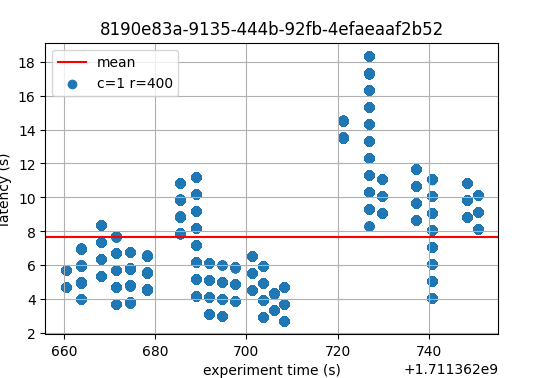
The figure below shows the values obtained for v1 and v0.38 (the baseline). It’s important to note
that configurations that have the same amount of total transaction load are regarded as equivalent.
For example, c=1,r=400 and c=2,r=200 are plotted on the same x-axis value corresponding to their
total rate of 400 tx/s, which corresponds to configuration with c=1.
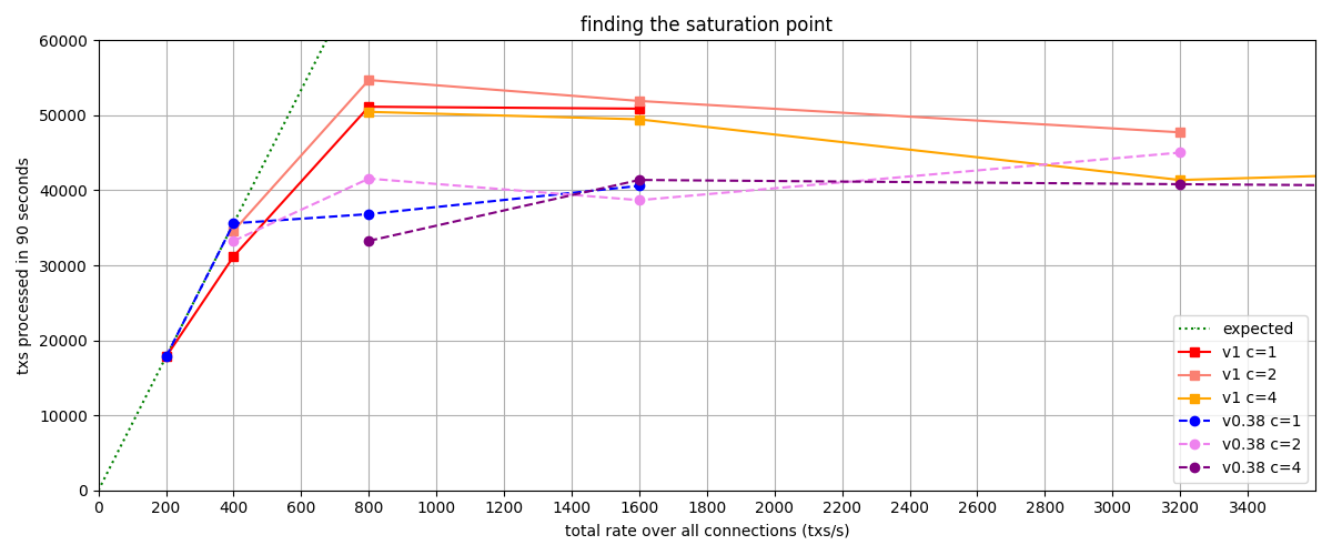
In the figure, we observe that up to a rate of 400 tx/s, the obtained values closely match or are
equal to the expected number of processed transactions, which is 35600 txs. However, beyond this
point, the system becomes overloaded and cannot process all incoming transactions, resulting in
dropped transactions. This state indicates that the system is saturated. The expected number of
processed transactions is calculated as c * r * 89 s = 35600 txs. It’s worth noting that we
utilize 89 out of 90 seconds of the experiment duration, as the final transaction batch coincides
with the end of the experiment and is thus not sent.
The complete results from which the figure was generated can be found in the file
v1_report_tabbed.txt. The following table summarizes the
values plotted in the figure, that is, the number of transaction processed. We can see the
saturation point in the diagonal defined by c=1,r=400 and c=2,r=200:
| r | c=1 | c=2 | c=4 |
|---|---|---|---|
| 200 | 17800 | 34600 | 50464 |
| 400 | 31200 | 54706 | 49463 |
| 800 | 51146 | 51917 | 41376 |
| 1600 | 50889 | 47732 | 45530 |
For comparison, this is the table obtained on the baseline version, with the same saturation point:
| r | c=1 | c=2 | c=4 |
|---|---|---|---|
| 200 | 17800 | 33259 | 33259 |
| 400 | 35600 | 41565 | 41384 |
| 800 | 36831 | 38686 | 40816 |
| 1600 | 40600 | 45034 | 39830 |
In conclusion, we chose c=1,r=400 as the transaction load that we will use in the rest of QA
process. This is the same value used in the previous QA tests.
With latency emulation
For comparing where the network starts to saturate in v1 with and without latency emulation, we
run a new set of experiments with different configurations of transaction loads: we use only one
connection and a transaction rate ranging from 100 to 1000 tx/s, in intervals of 100. The figure
depicts in total six instances of these experiments, three with latency emulation and three without.
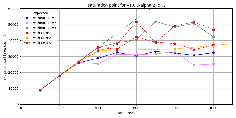
Up to 300 tx/s, the throughput is optimal for both configurations. However, when the load increases beyond this threshold, not all transactions are processed. Given the limited number of experiments conducted, it’s challenging to conclusively determine which configuration offers better throughput. Nevertheless, we can still say that there are no big discrepancies in the obtained values on both scenarios.
200-nodes test
This experiment consists in running the 200-nodes network, injecting a load of 400 tx/s (c=1,r=400)
during 90 seconds, and collecting the metrics. The network composition is the same as used for
finding the saturation point.
For the experiments with latency emulation we have set a duration of 180 seconds instead of 90.
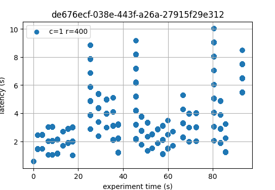
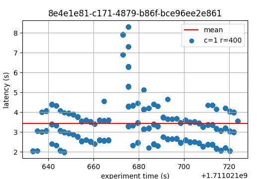
Latencies
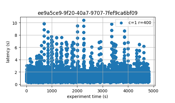
The following figures show the latencies of the experiment. Each dot represents a block: at which time it was created (x axis) and the average latency of its transactions (y axis).
| v0.38 | v1 (without LE / with LE) |
|---|---|
 |
 |
 |
In both cases, most latencies are around or below 4 seconds. On v0.38 there are peaks reaching 10
seconds, while on v1 (without LE) the only peak reaches 8 seconds. Even if both images are
similar, it’s crucial to note that v0.38 implements BFT time, while the experiments on
v1 were performed with PBTS. The implication is that PBTS tends to produce slightly
smaller latencies. The reason is that, in PBTS, the block’s timestamp is the proposer’s wallclock
value at the moment the block was created. For reference, with BFT time, the block’s timestamp is
the median of the timestamp of all precommits in the previous height. Each of these timestamps
reflects the validator’s wallclock time when the precommit is sent. Consequently, latencies
calculated when BFT time is active tend to contain one extra network propagation delay–the one
whereby precommits are disseminated.
With these considerations in mind, and taking into account that this is a small experiment, we infer
that the latencies measured on v1 are not worse than those of the baseline. With latency
emulation, the latencies are considerably higher, as expected.
Metrics
In this section we analyse key metrics extracted from Prometheus data on the 200-nodes experiment
with configuration c=1,r=400.
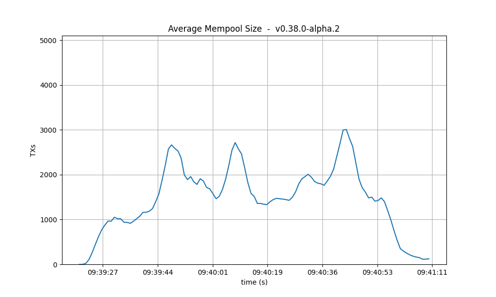
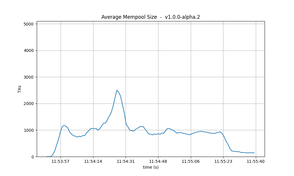
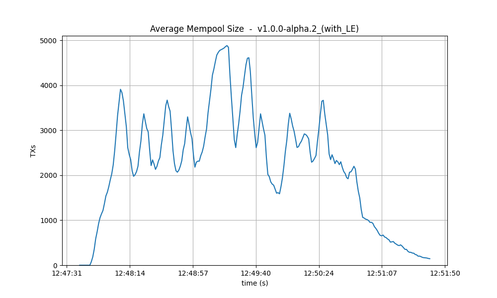
Mempool size
The following figures show the evolution of the average and maximum mempool size over all full nodes.
Average size On v1, the average mempool size mostly stays below 1000 outstanding transactions
except for a peak above 2000, coinciding with the moment the system reached round number 1 (see
below). For these particular runs, this result is better than the baseline, which oscilates between
1000 and 2500.
With latency emulation, the average mempool size stays mostly above 2000 outstanding transactions with peaks almost reaching the maximum mempool size of 5000 transactions.
| v0.38 | v1 (without LE / with LE) |
|---|---|
 |
 |
 |
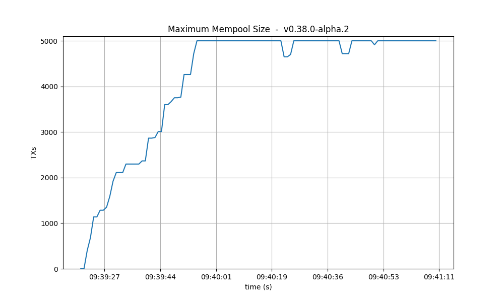
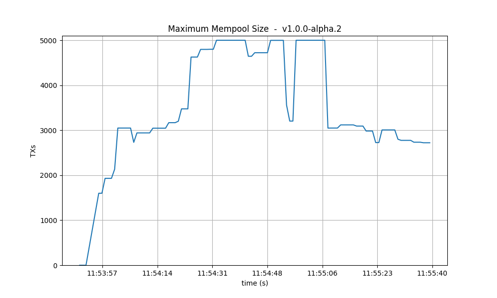
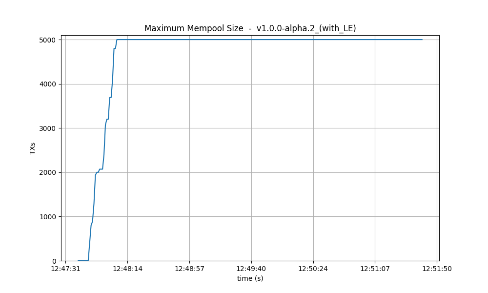
Maximum size The maximum mempool size indicates when one or more nodes have reached their
maximum capacity in terms of the number of transactions they can hold. In version v0.38, it’s
apparent that most of the time, at least one node is dropping incoming transactions.
Conversely, in v1, this happens less often, especially after reaching round 1 (as detailed below).
However, when we introduce latency emulation into v1, there is consistently at least one node with
a saturated mempool.
| v0.38 | v1 (without LE / with LE) |
|---|---|
 |
 |
 |
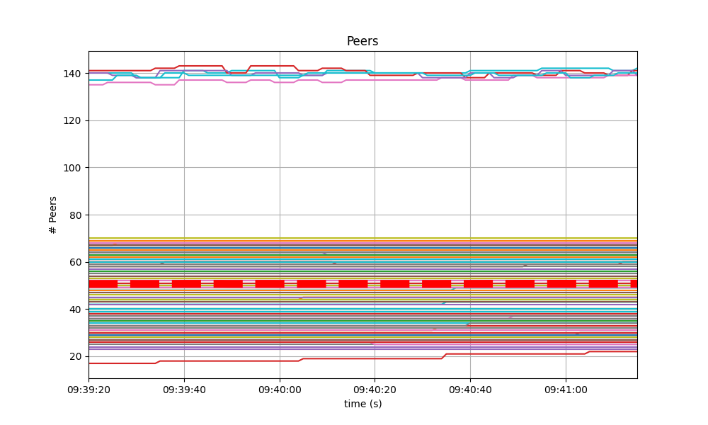
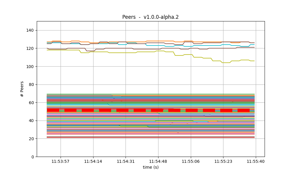
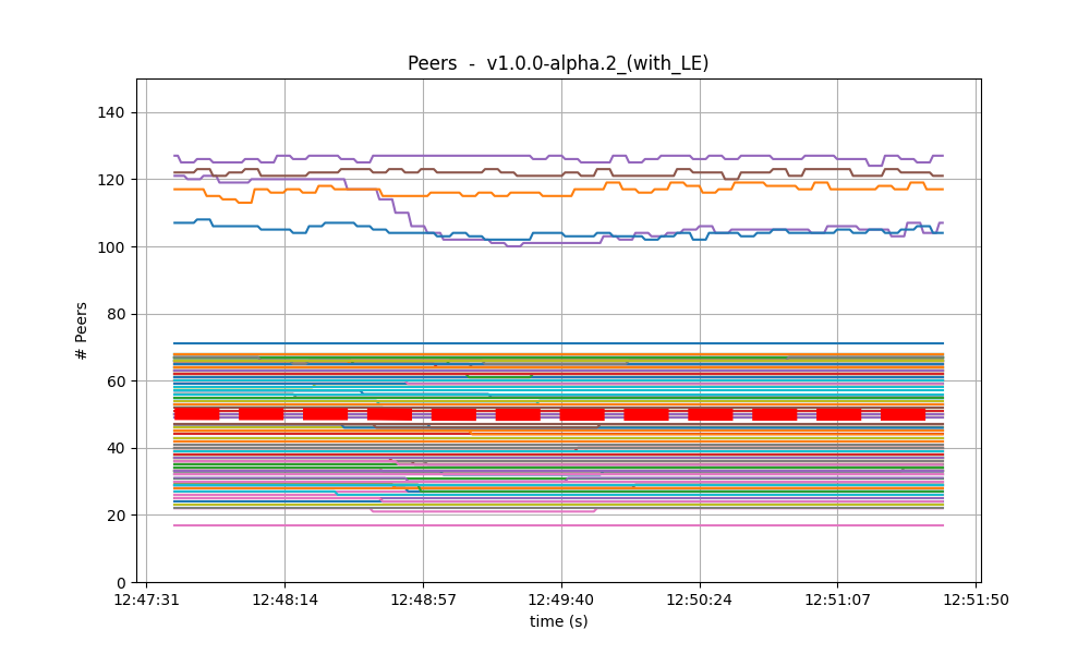
Peers
On all experiments, the number of peers was stable on all nodes. As expected, the seed nodes have more peers (around 125) than the rest (between 20 and 70 for most nodes). The red dashed line denotes the average value. Just as in the baseline, the fact that non-seed nodes reach more than 50 peers is due to [#486].
| v0.38 | v1 (without LE / with LE) |
|---|---|
 |
 |
 |
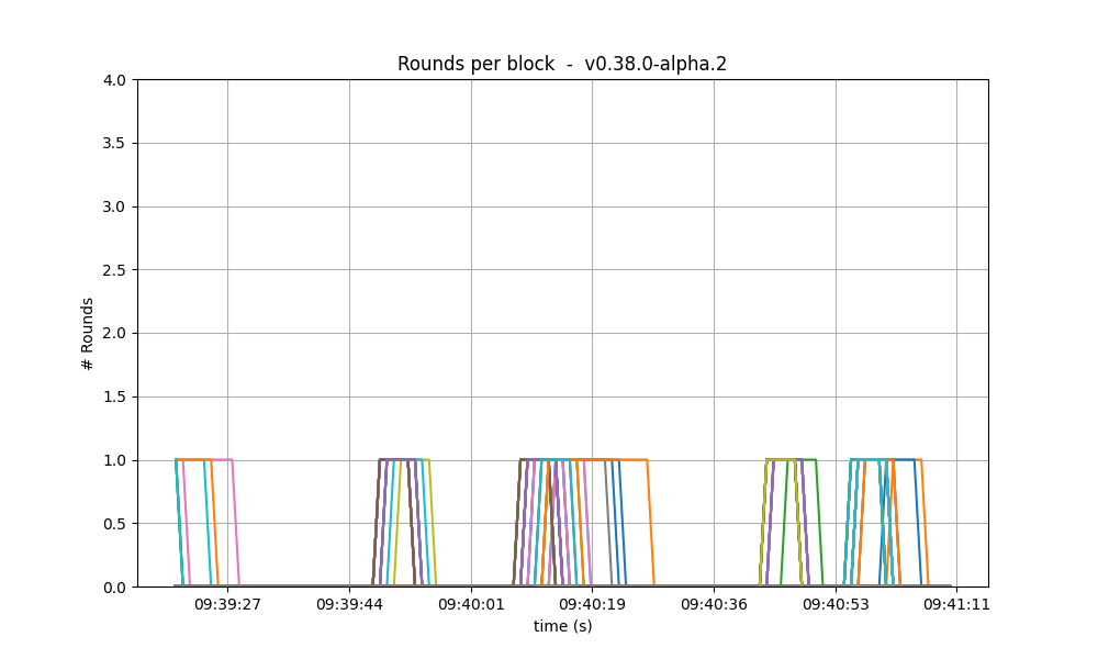
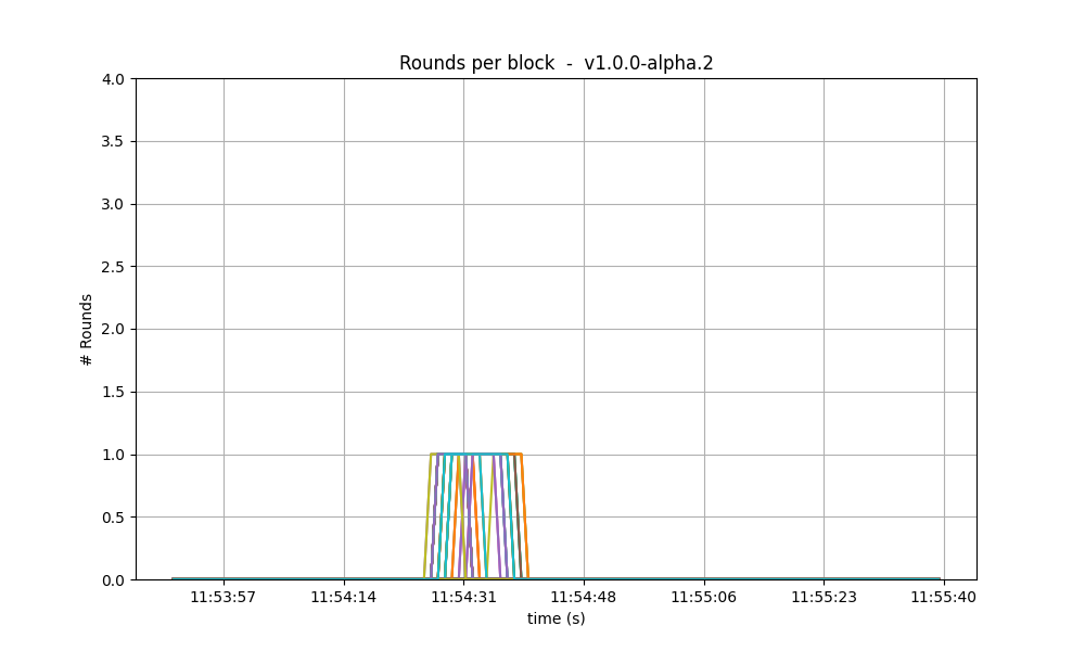
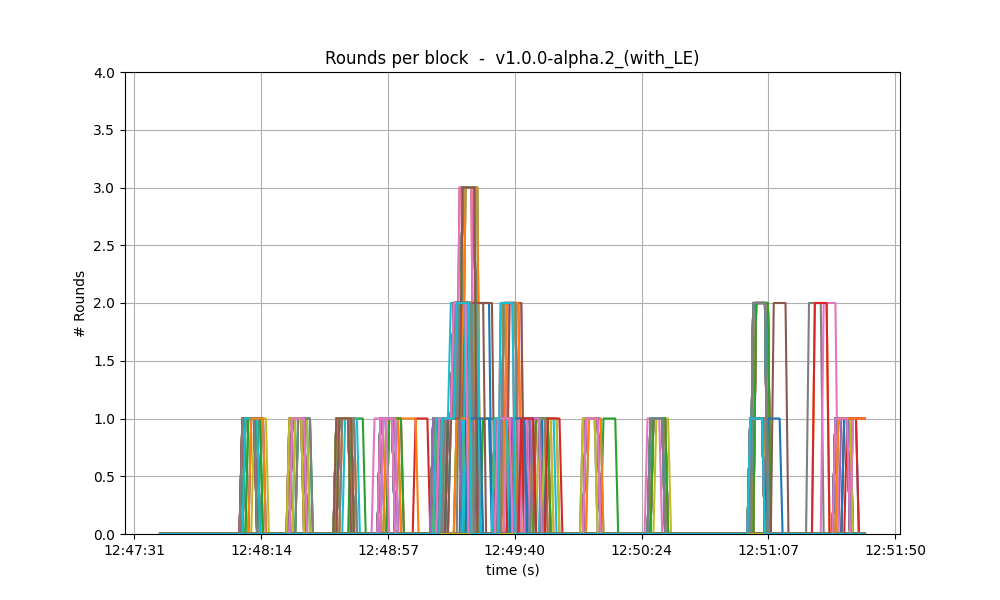
Consensus rounds
On both versions, most blocks took just one round to reach consensus, except for a few cases when
a second round was needed. On these two particular runs, we observe that v0.38 required an extra
round on more occasions than v1.
With latency emulation, the performance is notably worse: the consensus module requires an extra round more often, even needing four rounds to finalise a block. This indicates that the values of consensus timeouts should be increased, so that to represent the actual delays in the network.
| v0.38 | v1 (without LE / with LE) |
|---|---|
 |
 |
 |
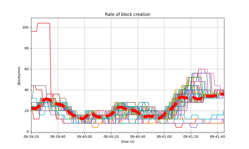
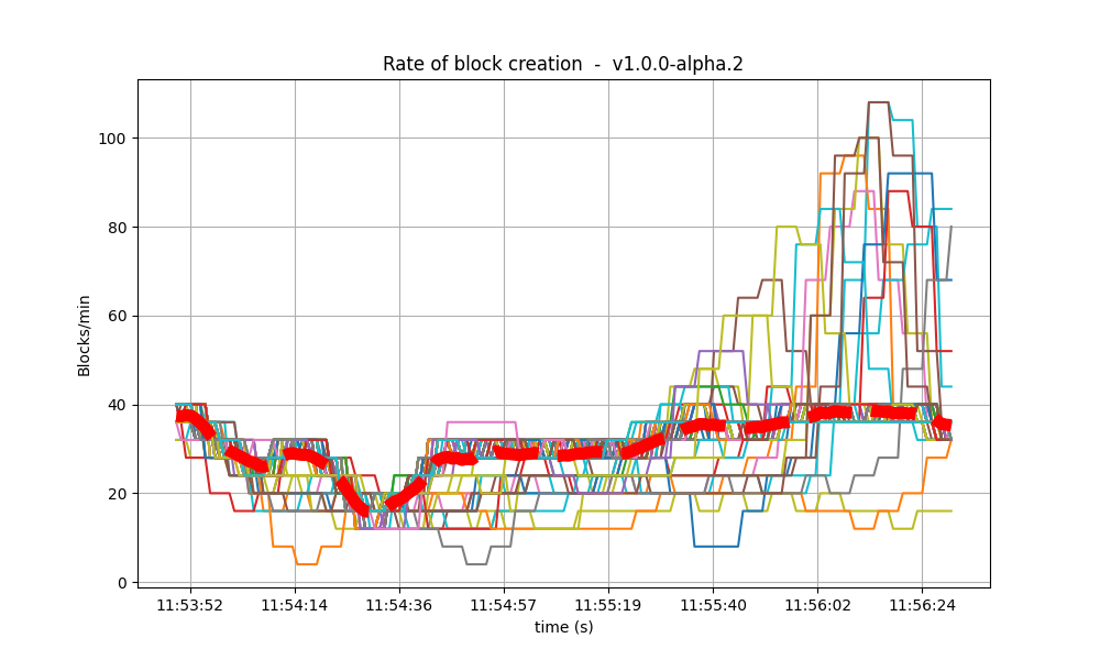
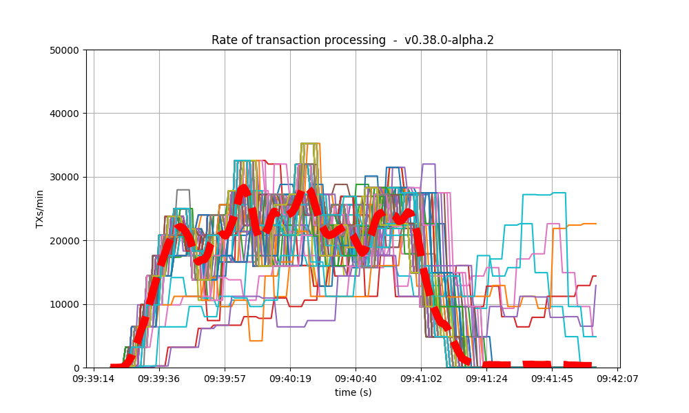
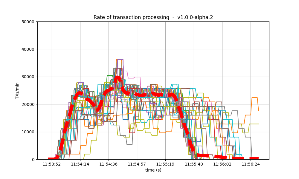
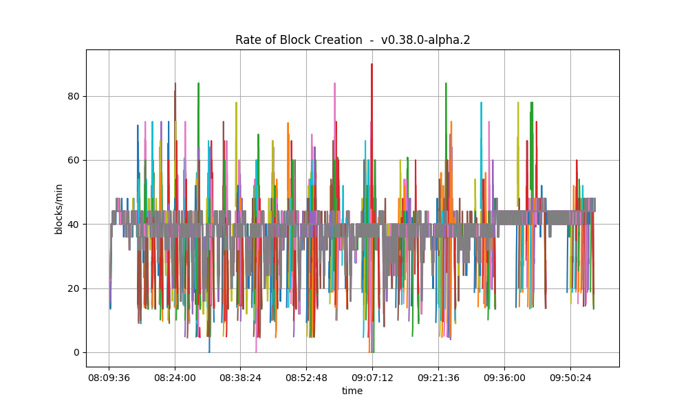
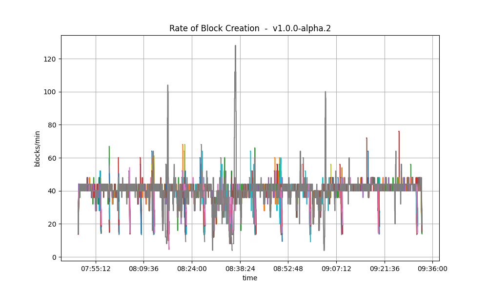
Blocks produced per minute and transactions processed per minute
These figures show the rate in which blocks were created from the point of view of each node, indicating when each node learned that a new block had been agreed upon. Throughout much of the load application period, the majority of nodes maintained a rate of between 20 and 40 blocks per minute. A spike to more than 100 blocks per minute occurred due to a slower node catching up. In the baseline scenario, most blocks had a somewhat slower rate of approximately between 10 and 30 blocks per minute.
| v0.38 | v1 (without LE / with LE) |
|---|---|
 |
 |
 |
| v0.38 | v1 (without LE / with LE) |
|---|---|
 |
 |
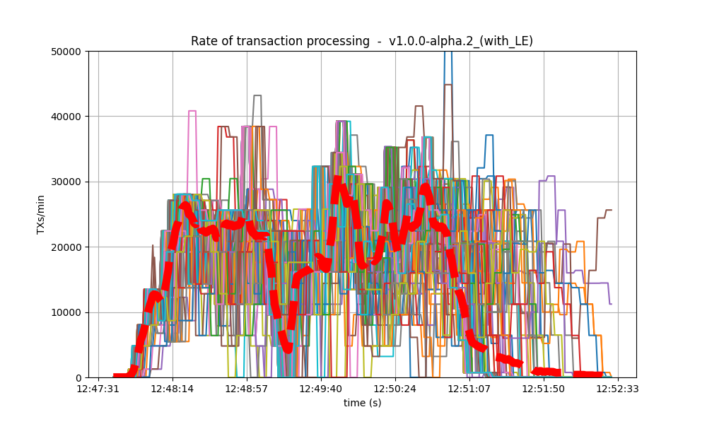 |
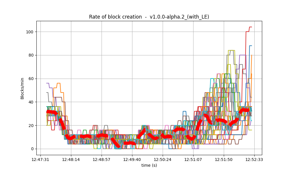
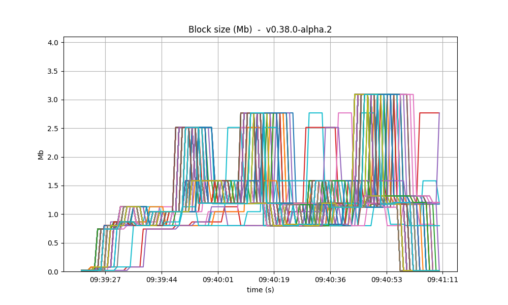
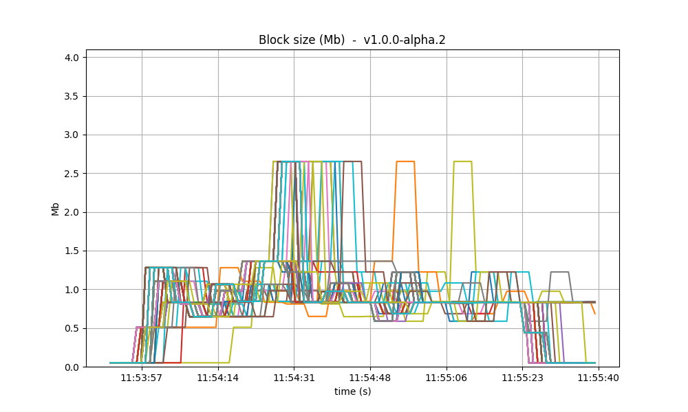
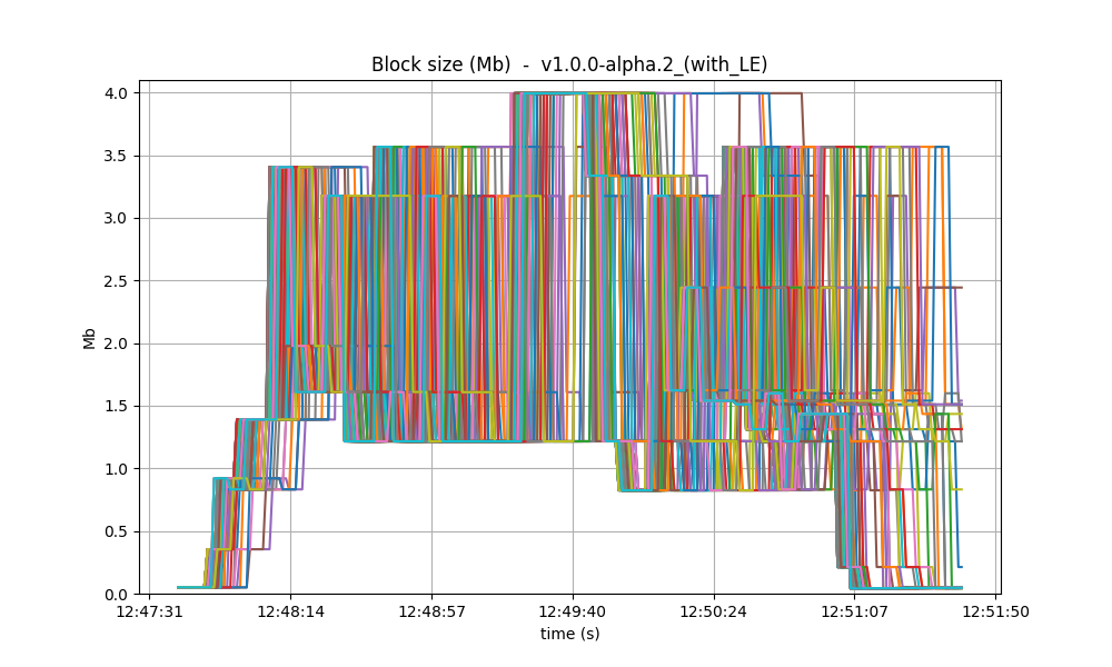
The collective spike on the right of the graph marks the end of the load injection, when blocks become smaller (empty) and impose less strain on the network.
With latency emulation (LE), there is a noticeable degradation in throughput. The block generation rate drops from approximately 30 blocks per minute (without LE) to around 10 blocks per minute. Since the rates of transaction processing are similar, this means that more transactions are included in the blocks, as shown in the following images. The most probable reason is that, once block latency is higher with latency emulation, more transactions are available at the proposer when it is ready to propose a new block. Note that the maximum block size is 4 Mb.
| v0.38 | v1 (without LE / with LE) |
|---|---|
 |
 |
 |
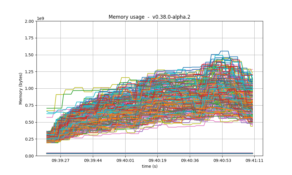
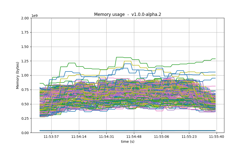
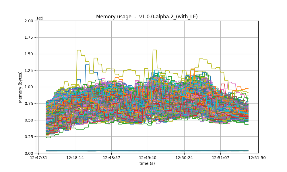
Memory resident set size
The following graphs show the Resident Set Size of all monitored processes. Most nodes use less than
0.9 GB of memory, and a maximum of 1.3GB. In all cases, the memory usage in v1 is less than in the
baseline. On all processes, the memory usage went down as the load was being removed, showing no
signs of unconstrained growth. With latency emulation, the results are comparable.
| v0.38 | v1 (without LE / with LE) |
|---|---|
 |
 |
 |
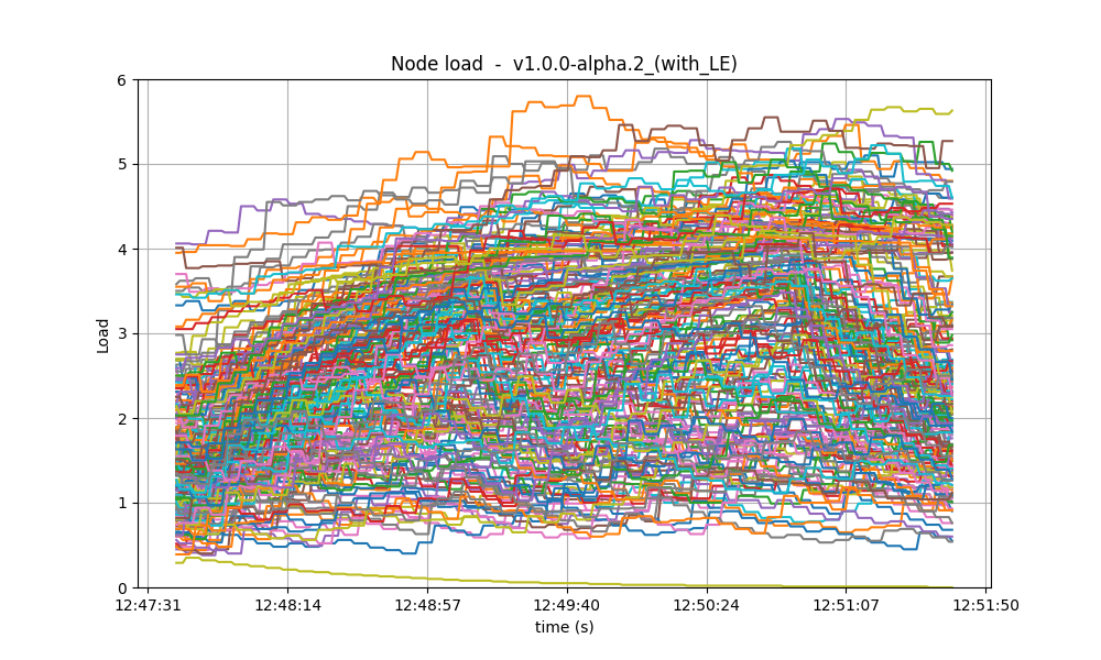
CPU utilization
The most reliable metric from Prometheus for assessing CPU utilization in a Unix machine is load1,
commonly found in the output of
top. In these scenarios,
the load remains consistently below 4 on the majority of nodes, with the baseline exhibiting a
similar pattern. With latency emulation, the CPU load reaches 5 on some nodes, probably due to
having a busier mempool and processing more rounds.
| v0.38 | v1 (without LE / with LE) |
|---|---|
 |
 |
 |
Test Results
We have demonstrated that there are no regressions when comparing CometBFT v1.0.0-alpha.2 against
the results obtained for v0.38. In fact, the observed results are identical to, or occasionally even
slightly better than those of the baseline. We therefore conclude that this version of CometBFT has
passed the test.
| Scenario | Date | Version | Result |
|---|---|---|---|
| 200-nodes | 2024-03-21 | v1.0.0-alpha.2 (4ced46d3d742bdc6093050bd67d9bbde830b6df2) | Pass |
Test results with latency emulation
As expected, the introduction of emulated latencies to the network results in a degradation of
performance for v1 compared to v1 without latency emulation, although not by an order of
magnitude. Moving forward with the next QA tests, it may be prudent to consider adjusting the
saturation point to a slightly lower value. Determining this adjustment will require conducting new
experiments on the network with latency emulation.
Rotating Nodes Testnet
As done in past releases, we use c=1,r=400 as load, as the saturation point in the 200-node test
has not changed from v0.38.x (see the corresponding section above).
Further, although latency emulation is now available, we decided to run this test case
without latency emulation (LE); this choice may change in future releases.
The baseline considered in this test case is v0.38.0-alpha.2, as described
in the introduction above.
Latencies
The following two plots show latencies for the whole experiment.
We see the baseline (v0.38.0-alpha.2) on the left, and the current version
on the right.
We can appreciate that most latencies are under 4 seconds in both cases, and both graphs have a comparable amount of outliers between 4 seconds and 11 seconds.
| v0.38.0 | v1.0.0 (without LE) |
|---|---|
 |
 |
Prometheus Metrics
This section shows relevant metrics both on v1.0.0 and the baseline (v0.38.0).
In general, all metrics roughly match those seen on the baseline
for the rotating node experiment.
Blocks and Transactions per minute
The following two plots show the blocks produced per minute. In both graphs, most nodes stabilize around 40 blocks per minute.
| v0.38.0 | v1.0.0 (without LE) |
|---|---|
 |
 |
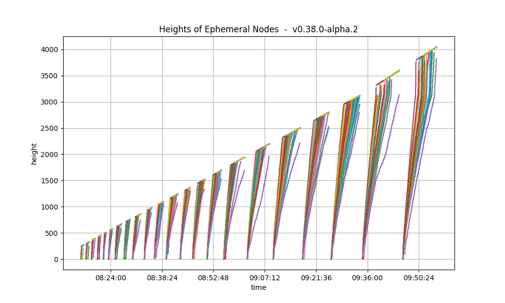
The following plots show only the heights reported by ephemeral nodes, both when they were blocksyncing and when they were running consensus.
| v0.38.0 | v1.0.0 (without LE) |
|---|---|
 |
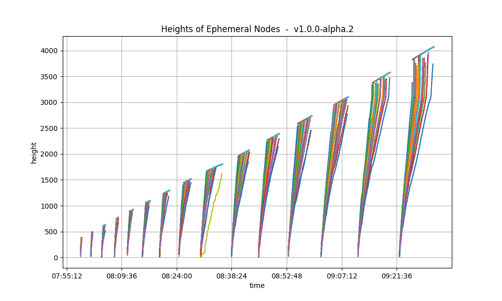 |
In both cases, we see the main loop of the rotating test case repeat itself a number of times.
Ephemeral nodes are stopped, their persisted state is wiped out, their config is transferred over
from the orchestrating node, they are started, we wait for all of them to catch up via blocksync,
and the whole cycle starts over. All these steps are carried out via ansible playbooks.
We see that there are less cycles in v1.0.0. The reason is the following.
All ansible steps are currently run from the orchestrating node (i.e., the engineer’s laptop).
The orchestrating node when running the rotating nodes test case for v1.0.0
was connected to a network connection that was slower than when the equivalent test was run for v0.38.x.
This caused the steps reconfiguring ephemeral nodes at the end of each cycle to be somewhat slower.
This can be noticed in the graphs when comparing the width (in x-axis terms) of the gaps without metric
from the end of a cycle to the beginning of the next one.
If we focus on the width of periods when ephemeral nodes are blocksynching, we see that they are slightly narrower
in v1.0.0. This is likely due to the improvements introduced as part of the issues
#1283,
#2379, and
#2465.
The following plots show the transactions processed per minute.
| v0.38.0 | v1.0.0 (without LE) |
|---|---|
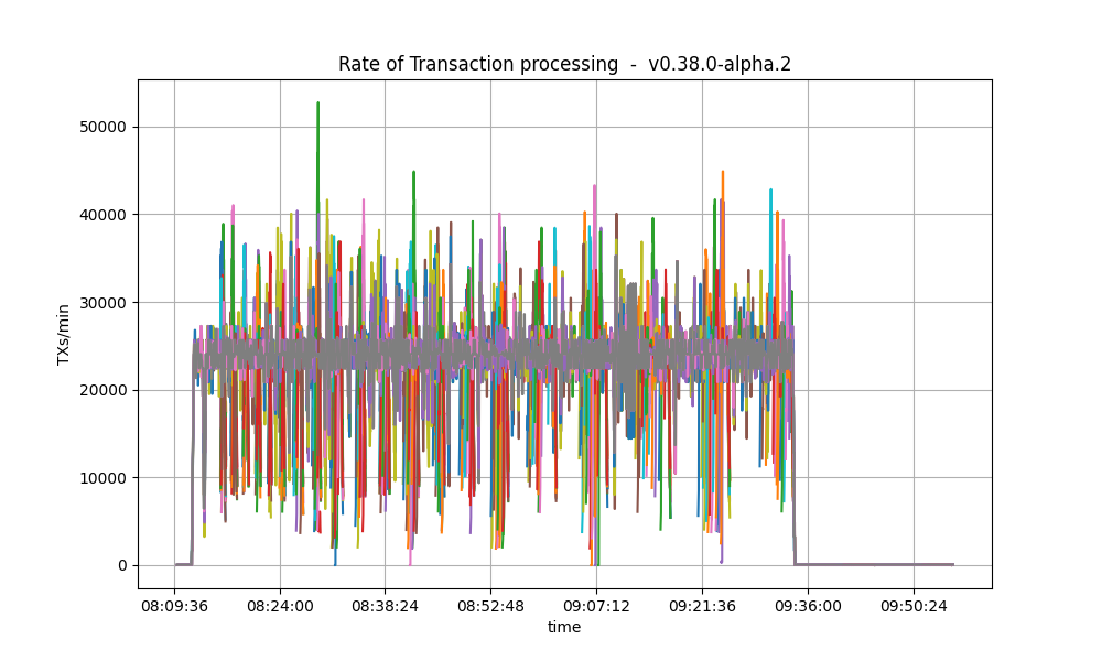 |
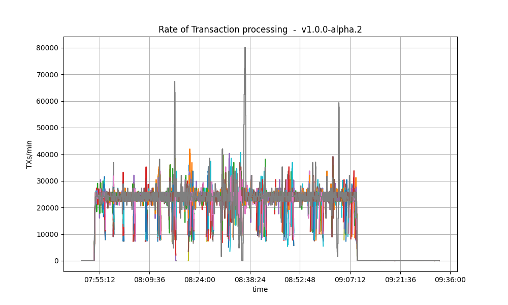 |
They seem similar, except for an outlier in the v1.0.0 plot.
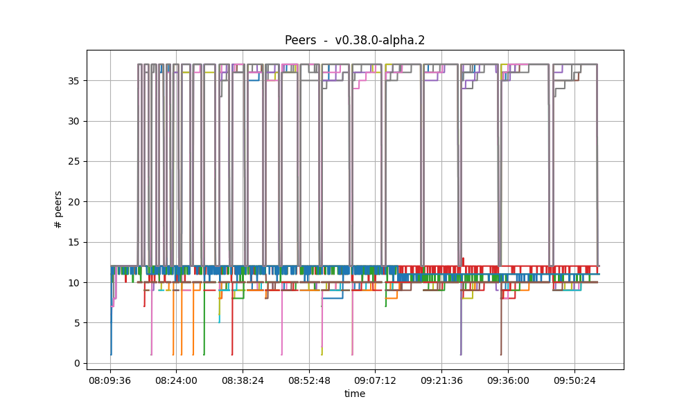
Peers
The plots below show the evolution of the number of peers throughout the experiment.
| v0.38.0 | v1.0.0 (without LE) |
|---|---|
 |
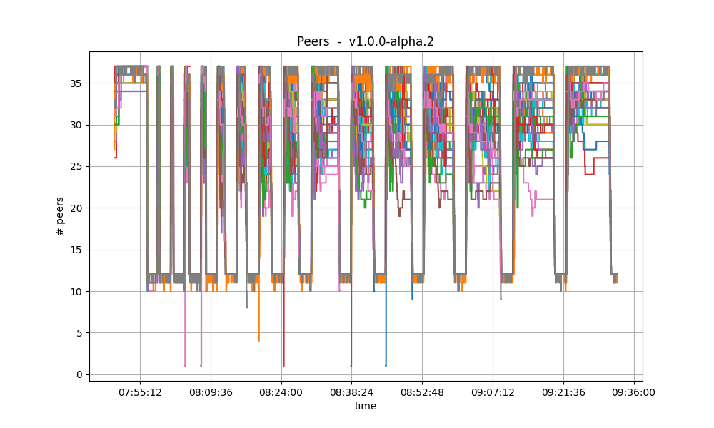 |
The plotted values and their evolution show the same dynamics in both plots.
Nevertheless, all nodes seem to acquire more peers when ephemeral node are catching up in the v1.0.0 experiment.
For further explanations on these plots, see the this section.
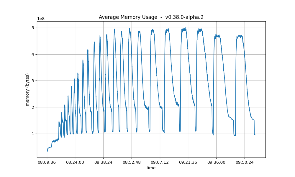
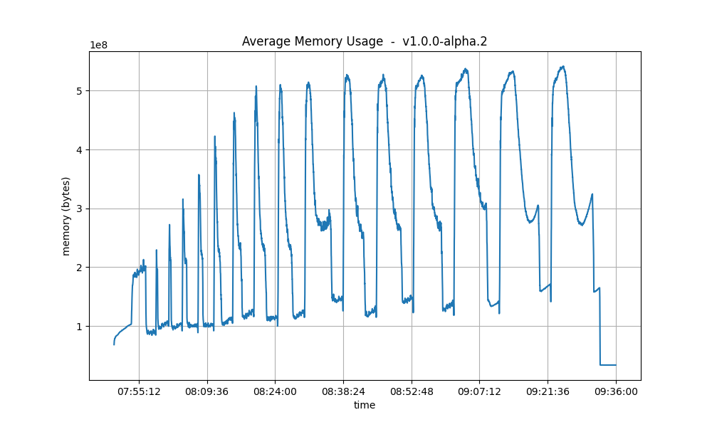
Memory Resident Set Size
These plots show the average Resident Set Size (RSS) over all processes. They are comparable in both releases.
| v0.38.0 | v1.0.0 (without LE) |
|---|---|
 |
 |
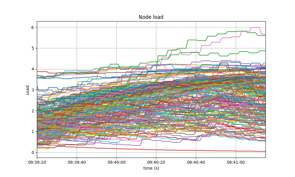
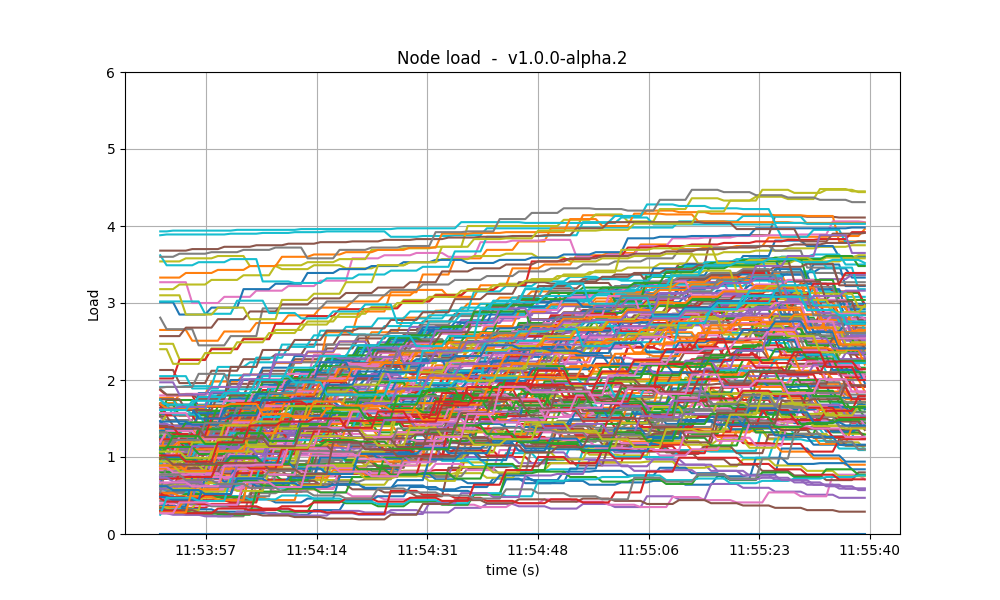
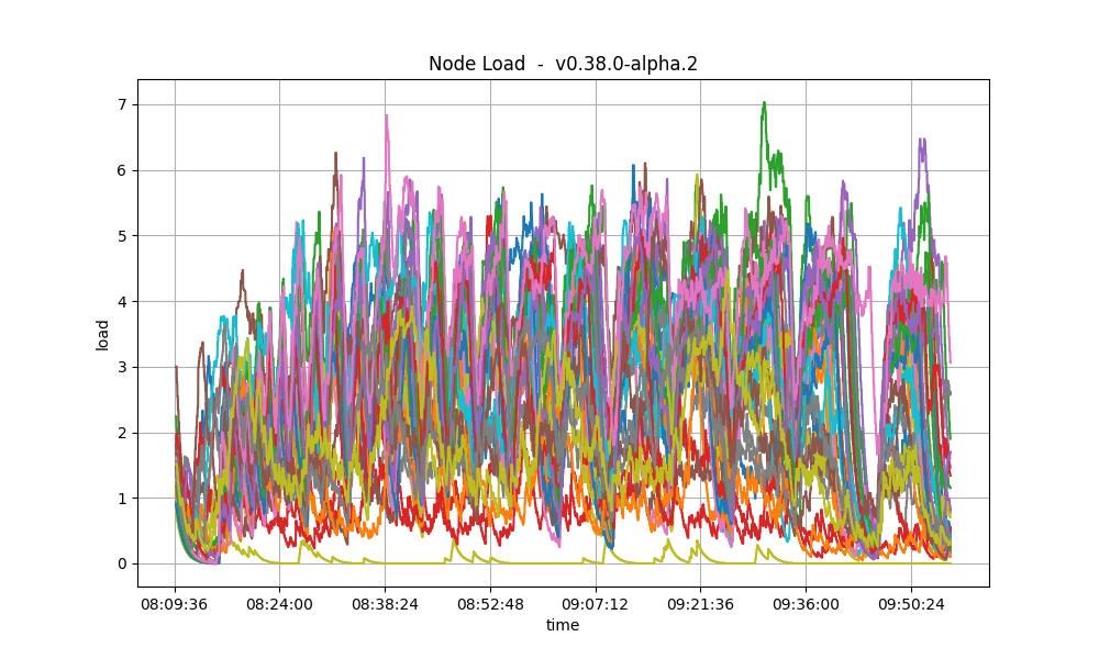
CPU utilization
The plots below show metric load1 for all nodes for v1.0.0-alpha.2 and for the baseline (v0.38.0).
| v0.38.0 | v1.0.0 (without LE) |
|---|---|
 |
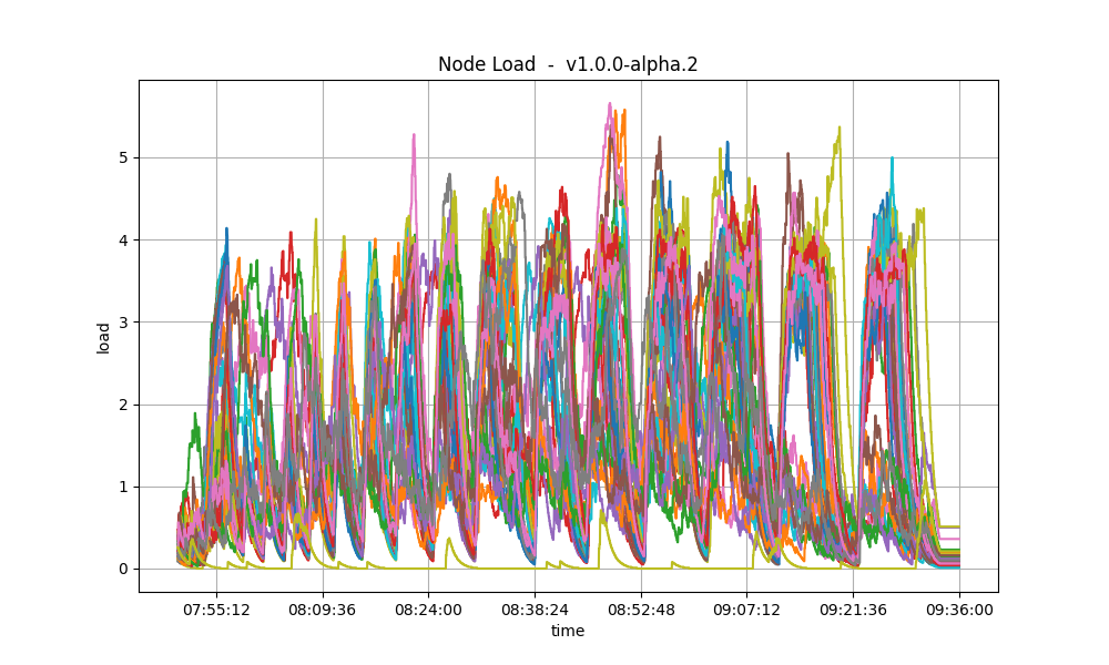 |
In both cases, it is contained under 5 most of the time, which is considered normal load.
Test Result
| Scenario | Date | Version | Result |
|---|---|---|---|
| Rotating | 2024-04-03 | v1.0.0-alpha.2 (e42f62b681a2d0b05607a61d834afea90f73d366) | Pass |
